ASSET: Analysis of Sequences of Synchronous Events in Massively Parallel Spike Trains
The tutorial is based on the paper [1] and demonstrates a method of finding patterns of synchronous spike times (synfire chains) which cannot be revealed by measuring neuronal firing rates only.
In this tutorial, we use 50 neurons per group in 10 successive groups of a synfire chain embedded in a balanced network simulation. For more information about the data and ASSET algorithm, refer to [1].
References
[1] Torre E, Canova C, Denker M, Gerstein G, Helias M, Grün S (2016) ASSET: Analysis of Sequences of Synchronous Events in Massively Parallel Spike Trains. PLoS Comput Biol 12(7): e1004939. https://doi.org/10.1371/journal.pcbi.1004939
1. Explore the data and postulate the problem
We start by importing the required packages, setting up matplotlib and loading the data.
[1]:
import matplotlib.pyplot as plt
import numpy as np
import quantities as pq
import neo
import elephant
from elephant import asset
[2]:
%load_ext autoreload

plt.style.use('dark_background')

plt.rcParams['figure.autolayout'] = False
plt.rcParams['figure.figsize'] = 20, 12
plt.rcParams['axes.labelsize'] = 18
plt.rcParams['axes.titlesize'] = 20
plt.rcParams['font.size'] = 14
plt.rcParams['lines.linewidth'] = 1.0
plt.rcParams['lines.markersize'] = 8
plt.rcParams['legend.fontsize'] = 14

plt.rcParams['text.latex.preamble'] = r"\usepackage{subdepth}, \usepackage{type1cm}"
plt.rcParams['mathtext.fontset'] = 'cm'
First, we download the data, packed in NixIO structure, from https://gin.g-node.org/INM-6/elephant-data
[3]:
!wget -N https://web.gin.g-node.org/INM-6/elephant-data/raw/master/dataset-2/asset_showcase_500.nix
The data is represented as a neo.Block with one neo.Segment inside, which contains raw neo.SpikeTrains. For more information on neo.Block, neo.Segment, and neo.SpikeTrain refer to https://neo.readthedocs.io/en/stable/core.html
[4]:
with neo.NixIO('asset_showcase_500.nix', 'ro') as f:
    block = f.read_block()
segment = block.segments[0]
spiketrains = segment.spiketrains
[5]:
plt.figure()
plt.eventplot([st.magnitude for st in spiketrains], linewidths=5, linelengths=5)
plt.xlabel('time [ms]')
plt.ylabel('neuron id')
plt.title('Raw spikes')
plt.show()
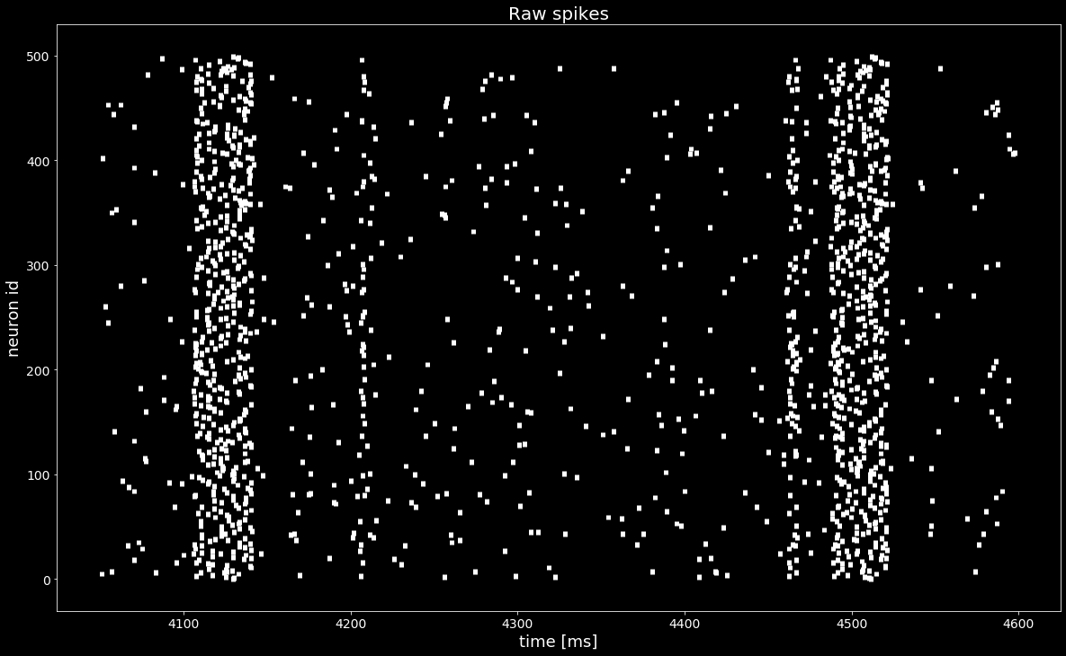
Even though we see an increase of the firing rate, we cannot find a propagating activity just by looking at the raster plot above.
We want to find a permuation of rows (neurons) in spiketrains such that a pattern (synfire chain) appears. The true unknown permutation is stored in the segment.annotations['spiketrain_ordering']. The goal is to recreate this permutation from raw data with the statistical method ASSET.
2. Applying ASSET
2.1. Intersection matrix
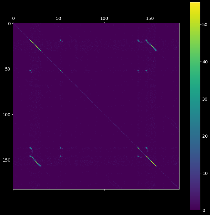
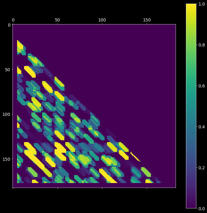
The first step is to compute the intersection matrix imat, the (i,j) entry of which represents the number of neurons spiking both at bins i and j after the binning is applied. The resultant symmetric matrix imat shows one off-diagonal synfire chain pattern (see the picture below).
[6]:
# 2.1.1) create ASSET analysis object
# hint: try different bin sizes, e.g. bin_size=2.5, 3.5, 4.0 ms
asset_obj = asset.ASSET(spiketrains, bin_size=3*pq.ms)

# 2.1.2) compute the intersection matrix
imat = asset_obj.intersection_matrix()
plt.matshow(imat)
plt.colorbar();
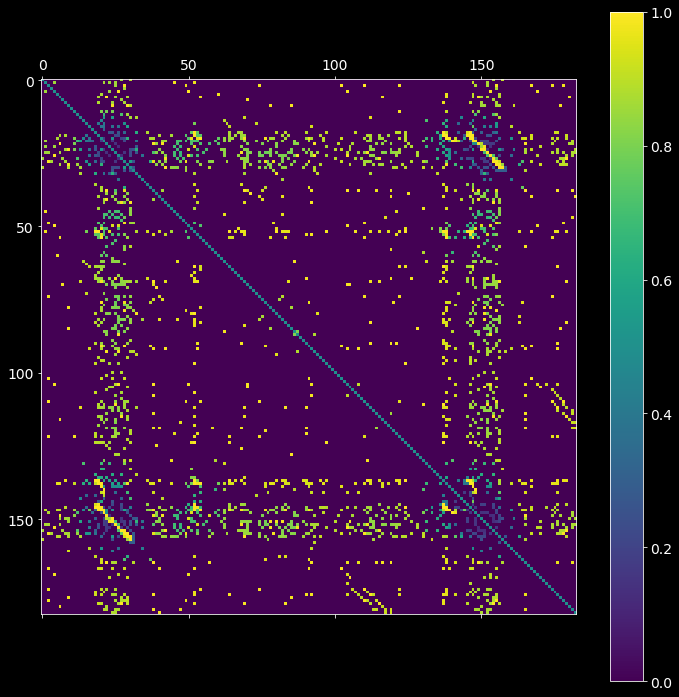
2.2. Analytical probability matrix
The second step is to estimate the probability  that non-zero entries in
 imat occurred by chance. The resultant pmat matrix is defined as the probability of having strictly fewer coincident spikes at bins i and j strictly than the observed overlap (imat) under the null hypothesis of independence of the input spike trains.
[7]:
pmat = asset_obj.probability_matrix_analytical(imat, kernel_width=50*pq.ms)
plt.matshow(pmat)
plt.colorbar();
compute rates by boxcar-kernel convolution...
compute the prob. that each neuron fires in each pair of bins...
compute the probability matrix by Le Cam's approximation...
substitute 0.5 to elements along the main diagonal...
2.3. Joint probability matrix
The third step is postprocessing of the analytical probability matrix pmat, obtained from the previous step. Centered at each (i,j) entry of pmat matrix, we apply a diagonal kernel with shape filter_shape and select the top nr_largest probabilities of (i,j) neighborhood (defined by filter_shape), and compute the significance of these nr_largest joint neighbor probabilities. The resultant jmat matrix is a “dilated” version of imat.
This step is most time consuming.
[8]:
# hint: try different filter_shapes, e.g. filter_shape=(7,3)
jmat = asset_obj.joint_probability_matrix(pmat, filter_shape=(11, 3), n_largest=3)
Joint survival function: 100%|██████████| 47838/47838 [00:06<00:00, 7400.11it/s]
[9]:
plt.matshow(jmat)
plt.colorbar();
2.4. Mask matrix
After setting significance thresholds  and
and  for the corresponding matrices
  (probability matrix
 pmat) and  (joint probability matrix
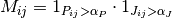
 jmat), we check the entries for significance. The resultant boolean mask matrix mmat is then defined as
[10]:
# hint: try different alphas for pmat and jmat
# hint: try alphas in range [0.99, 1-1e-6]
# hint: you can call 'asset.ASSET.mask_matrices(...)' without creating the asset_obj
alpha = .99
mmat = asset_obj.mask_matrices([pmat, jmat], [alpha, alpha])
plt.matshow(mmat);
2.5. Find clusters in the mask matrix
Each entry (i,j) of the mask matrix  from the previous step is assigned to a cluster id. A cluster is constrained to have at least
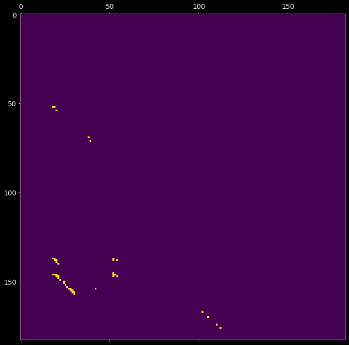
 min_neighbors number of associated elements with at most eps intra-distance (within the group). The cluster index, or the (i,j) entry of the resultant cmat matrix, is:
- a positive int (cluster id), if (i,j) is part of a cluster;
0, if is non-positive;
-1, if the element (i,j) does not belong to any cluster.
[11]:
# hint: you can call asset.ASSET.cluster_matrix_entries(...) without creating the asset_obj
cmat = asset_obj.cluster_matrix_entries(mmat, max_distance=11, min_neighbors=10, stretch=5)
plt.matshow(cmat)
plt.colorbar();
2.6. Sequences of synchronous events
Given the input spike trains, two arrays of bin edges from step 2.2 and the clustered intersection matrix cmat from step 2.5, extract the sequences of synchronous events (synfire chains).
[12]:
sses = asset_obj.extract_synchronous_events(cmat)
sses.keys()
[12]:
dict_keys([1])
[13]:
cluster_id = 1
cluster_chain = []
for chain in sses[cluster_id].values():
    cluster_chain.extend(chain)

_, st_indices = np.unique(cluster_chain, return_index=True)
st_indices = np.take(cluster_chain, np.sort(st_indices))

reordered_sts = [spiketrains[idx] for idx in st_indices]
spiketrains_not_a_pattern = [spiketrains[idx] for idx in range(len(spiketrains))
                      if idx not in st_indices]
reordered_sts.extend(spiketrains_not_a_pattern)
[14]:
plt.figure()
plt.eventplot([st.magnitude for st in reordered_sts], linewidths=5, linelengths=5)
plt.xlabel('time [ms]')
plt.ylabel('reordered neuron id')
plt.title('Reconstructed ordering of the neurons (y-axis) with synfire chains');
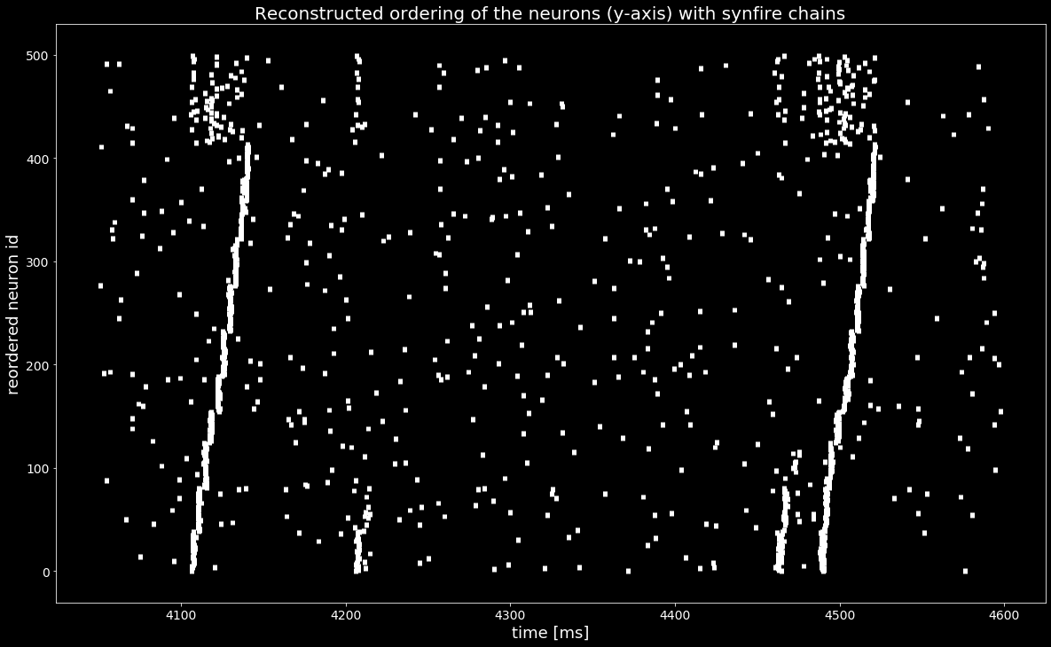
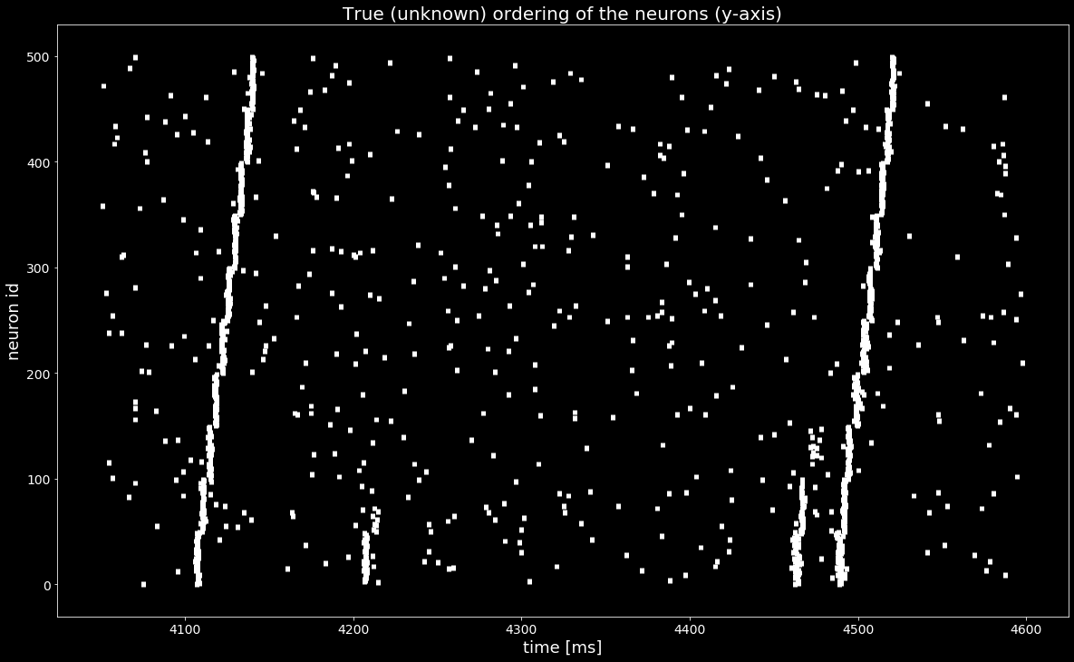
With the sequences of synchronous events sses we found a permutation of the spiketrains that reveals the synfire chain as in the ground truth ordering in the last Figure, shown below..
[15]:
ordering_true = segment.annotations['spiketrain_ordering']
spiketrains_ordered = [spiketrains[idx] for idx in ordering_true]

plt.figure()
plt.eventplot([st.magnitude for st in spiketrains_ordered], linewidths=5, linelengths=5)
plt.xlabel('time [ms]')
plt.ylabel('neuron id')
plt.title('True (unknown) ordering of the neurons (y-axis)')
plt.show()